Interpreting the Gaussian Output File
1. The Scan Specification Is Echoed
Near the start of the job, Gaussian confirms how it parsed the scan request:
!       B3          0.9      Scan                                      !
------------------------------------------------------------------------
Trust Radius=3.00D-01 FncErr=1.00D-07 GrdErr=1.00D-06
Number of optimizations in scan=  11
Number of steps in this run=     34 maximum allowed number of steps=   100.
Number of optimizations in scan = 11 confirms the 11 scan points requested (10 steps beyond the starting value). Number of steps in this run = 34 is the total count of geometry-optimization steps needed across all 11 points combined, it varies scan point to scan point, since each optimization runs until its own convergence criteria are met.
2. Each Scan Point Is a Full Optimization
Step number   1 out of a maximum of   34 on scan point     1 out of    11
...
SCF Done:  E(RB3LYP) =  -379.397996643     A.U. after   15 cycles
For every one of the 11 values of B3, Gaussian runs a complete Berny geometry optimization over all the unconstrained variables, printing an SCF energy at every optimization cycle. Later scan points typically converge faster than the first, since each one starts from the previous point's already-relaxed geometry rather than from scratch.
3. Stationary Point Confirmation
Once a scan point's optimization converges, Gaussian reports the stationary point and, alongside the fixed coordinate, the residual force along it (-DE/DX), the small remaining gradient component that the constraint is holding in check.
4. Summary of Optimized Potential Surface Scan
At the end of the job, Gaussian collects every point into a single table:
Summary of Optimized Potential Surface Scan

     Eigenvalues --  -379.39846-379.40225-379.40508-379.40708-379.40838
           B3           0.90000   0.92000   0.94000   0.96000   0.98000
     Eigenvalues --  -379.40910-379.40933-379.40916-379.40868-379.40796
           B3           1.00000   1.02000   1.04000   1.06000   1.08000
     Eigenvalues --  -379.40707
           B3           1.10000
Reading the two rows together gives the full energy profile:
| B3 (Å) | 0.90 | 0.92 | 0.94 | 0.96 | 0.98 | 1.00 | 1.02 | 1.04 | 1.06 | 1.08 | 1.10 |
|---|---|---|---|---|---|---|---|---|---|---|---|
| E (Hartree) | -379.39846 | -379.40225 | -379.40508 | -379.40708 | -379.40838 | -379.40910 | -379.40933 | -379.40916 | -379.40868 | -379.40796 | -379.40707 |
The energy drops steadily from 0.90 Å, bottoms out at B3 ≈ 1.02 Å (E = -379.40933 Hartree), and rises again toward 1.10 Å, a clean, single-minimum well. This locates the equilibrium O–H bond length at this level of theory and shows the energetic cost of stretching or compressing it away from equilibrium in either direction.
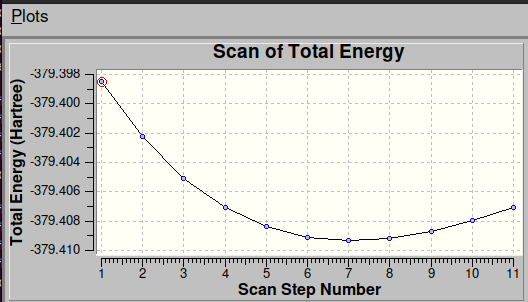
The energy profile from the table above, plotted against the scanned O–H bond length.
5. Job Completion
The orbital energies and population analysis that follow the scan summary belong to the last optimized point (B3 = 1.10 Å) and are the standard post-SCF output, unrelated to the scan itself.